Display
On the Display tab of the Stereonet Graph form, you can choose to:
- Show the density of the points rendered as a scattergram, or as contoured points,
- Calculate the Terzaghi Weighting.
- Show Grid lines, and
-
Set the Display Mode.
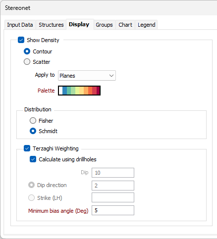
Show Density
Select this check box to select one of two Density Options (you can also select a Density Option from the Stereonet ribbon).


When there is a high density of data points it may be difficult to identify the zone where most of the data lies within the mass of points. This can be resolved by colour-coding each point according to the density of the points within its neighbourhood.
One of two modes of colour-coding may be applied:
- Contour - contour the points according to their relative density
- Scatter - colour-code each point according to the density of the points within its neighbourhood
Apply to
Choose whether the colour-coding is applied to the planes or the lineations.
Palette
Double-click on the Palette box to choose a palette. You can also right-click on the box to see a preview of the current palette.
Distribution
Choose a Distribution Option that best suits the data (you can also select a Distribution Option from the Stereonet ribbon).


Use the Fisher distribution to produce smoother contours of sparse data, and the Schmidt distribution to contour dense data. The difference between the two distributions decreases as the density of the data increases.
Terzaghi Weighting
The measurement of oriented structures always produces a bias in favour of those features which are perpendicular to the direction of surveying. Select this option to reduce that bias by applying a correction based upon the orientation in which the measurements were taken.
The effect of applying the Terzaghi weighting to data in unfavourable orientations can be quite severe and you should have a good understanding of the weighting procedure.
Calculate using drillholes
This option is enabled when the input to the process is an Event file. When the Calculate using drillholes check box is selected, a bias correction is applied using the orientation of the holes in the Drillhole Database.
Dip, Dip direction or Strike
When the Calculate using drillholes check box is not selected or enabled, you must define the direction of the scan-line by specifying a Dip and either a Dip Direction or a Strike.
Strike and dip notation is inconsistent and must include the handedness of the measurement to make it unambiguous. In this case, the handeness of the strike is assumed to be left-handed. A left-handed strike is one where the structure slopes downwards to the left when viewed along the direction of strike.
Minimum bias angle (in degrees)
The Minimum bias angle corresponds to the maximum possible weighting factor and is used to prevent the weighting factor from becoming excessively large. Any planes which intersect a traverse orientation at an angle less than the Minimum bias angle will be limited to the minimum angle. An initial bias angle of 15° is suggested.
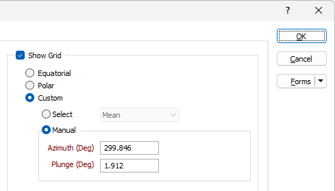
Show Grid
Select this check box to display a grid on the graph using the Grid Options (you can also select a Grid Option from the Stereonet ribbon).
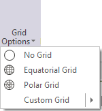
The grid can be based on an Equatorial or Polar stereographic projection, or a Custom projection.
If Custom is selected, you can choose Select and specify a grid calculation method from the drop down list:
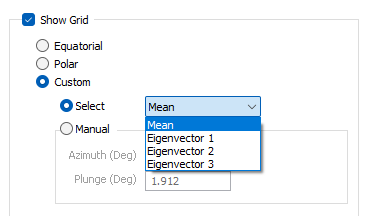
If you select the Manual option, you can manually specify the Plunge and Azimuth (in degrees) for the grid projection.
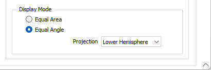
Display Mode
Select an option to display the Stereonet in one of two Display Modes (you can also select a Display Mode from the Stereonet ribbon).


Stereonets use the concept of an imaginary reference sphere, within which any structural measurement (in terms of plunge and trend) may be drawn as a line extending outward from its centre, eventually intersecting the sphere at two opposing points or poles.
For convenience the locations of these poles are then projected onto a horizontal plane passing through the centre of the reference sphere, cutting it into upper and lower hemispheres. Generally, only the lower hemisphere projection is used.
In an Equal Area projection the poles are projected as if they were peeled off the lower hemisphere, flattened, and then rescaled to match the reference sphere’s diameter.
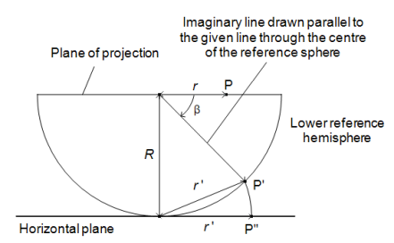
Vertical section through the centre of the lower reference hemisphere, illustrating an Equal Area projection.
In an Equal Angle projection the poles are projected by drawing a straight line from the pole to the top of the upper hemisphere, as if the viewer were looking downward from the north pole of the sphere.
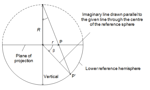
Vertical section through the centre of the lower reference hemisphere, illustrating an Equal Angle projection.
Reference: Priest S.D. (1985). Hemispherical Projection Methods in Rock Mechanics. George Allen and Unwin, London. 124 pp.